Precise GPS positions

Introduction

Normally GPS receivers available to civilians will give you a position that is good to about 15 meters. There is a military P (for Precise) code which does much better but  needs a special receiver which is not available to us muggles. Most modern GPS receivers use either an augmentation system (WAAS) or wifi and cell towers to provide additional information, improving accuracy to 2-3 meters. GPS receivers used for surveying use a second frequency to eliminate some of the errors. These can produce an accuracy of mm to cm but typically cost several thousand dollars/euros. So what can we do to get more precise GPS positions without putting on camo or spending lots of money ? Read on to see what can be done with more down-to-earth equipment.

Background on measurements

In order to get data that can get post-processed to get more precise positions, we need to enable a different type of messages from the GPS receiver. Normally GPS receivers output NMEA sentences which has information about the time, position and whether the receiver is moving. (NMEA was originally a standard for bits of boat  (the ‘M’ stands for ‘Marine’) electronics to talk to each other and was “borrowed” for GPS). These NMEA messages normally come from processing what is called the Coarse/Acquisition or C/A code. This code transmits 1 and 0’s at 1.023 million bits per  second. This means the code can transition from a 0 to 1 (or back again) in about:

Light travels about 0.3 meters in 1 ns (nanosecond) and the best we can measure the changing 1’s and 0’s in the C/A code is about 1 %. Combining all this we get:

As a related aside, the military P code is transmitted ten times faster (10.23 Mbps), which is part of the reason it is more accurate.

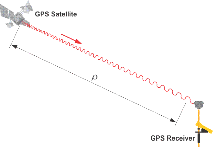
In order to get a position that is better than the standard available from the C/A code, we must measure what is known as the carrier phase.

This lets us measure to the same 1% of the changing signal, but this time the signal is the wavelength of the GPS L1 signal (about 19 cm). This means we can in principle measure the position to about 2mm. In order to do this, we need access to the raw signals of the pseudorange, carrier phase etc in the GPS receivers. Only certain GPS receivers make these raw signals available. The cheapest and most readily available for this are made by ublox.

Hardware needed

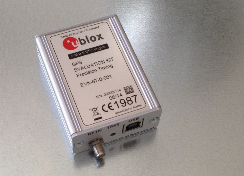
As mentioned above, we need a GPS receiver that allows us to record the raw measurements from the receiver for future post-processing. The ublox 6, 7 and M8N and M8T models can in theory output raw measurements. I have a ublox 6T as part of an evaluation kit (picture below) I got as part of a plan to build my own GPS Disciplined Oscillator (GPSDO); this last part hasn’t happened yet…

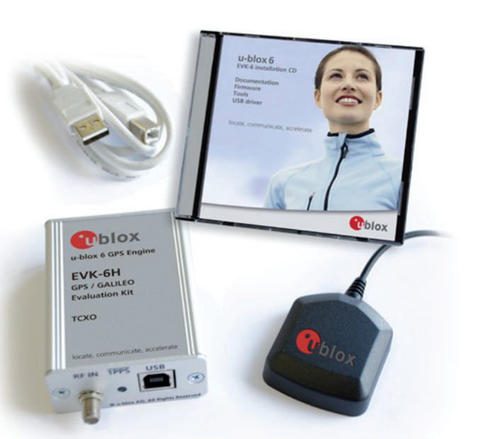
You will also need an antenna. My evaluation kit came with a patch antenna like the one in the picture below but any 5V antenna which can be connected (or converted) to a SMA connector will probably work. The ublox, like a lot of modern GPS receivers, is very sensitive and can get pretty good reception even indoors.

The quality of the precise GPS position you can get is going to depend on how many satellites you can see. This means the best results will be with a clear view of sky, particularly towards the South.

I now have a Symmetricom 58532A single frequency antenna mounted on the end of my house. This is connected with 100 feet of LMR240 cable through the attic and into my lab/office. This cable has a male Type N connector on the antenna end and a male SMA connector on the other. This goes through a 1 to 4 port Narda 4372a-4 splitter to feed the ublox (and other GPSes) via RG174 cables.

Software needed

RTKLIB

The software that is used to handle the capture and conversion is RTKLIB. It is recommended that you get the 2.4.3 beta version from github. This version has several years of additions over the standard 2.4.2 version. Instructions:

1. Go to https://github.com/tomojitakasu/RTKLIB/tree/rtklib_2.4.3, click on the ‘Clone or download’ button and then click on the ‘Download ZIP’ button. If you already have git installed (it’s available for Linux, Windows and Mac), then you can use the ‘Copy to clipboard’ icon and then download it with git clone <pasted url>.
2. Unless you want to compile from source (easy on Linux, harder on Mac), you probably want to grab the binaries as well. Go to https://github.com/tomojitakasu/RTKLIB_bin/tree/rtklib_2.4.3 and follow the same steps as above to download the zip or clone the repository.
3. You can either unpack this new zip file into the same directory as you unpacked to in Step 1. so that the bin/ directory is replaced with the actual binaries or leave it in a separate directory.

u-blox u-center

Before firing up the RTKLIB tools to gather data for the precise GPS positions, it is generally easiest to configure things in u-center. Once u-center has started up, go to View->Configuration View and you should see a window that looks like this:

I then perform the following changes to the settings (Remember to hit the ‘Send’ button at the bottom of the Configuration window after each step):

1. Under PRT (Ports), I set the  Target of 3 - USB to 0 - UBX under the Protocol Out section. This stops any of the normal NMEA messages coming out and confusing things.
2. Under TMODE (Time Mode), I set the Time Mode to 0 - Disabled. (This is only necessary if you have been using the GPS previously in static time mode).
3. You can configure the Messages needed under the MSG (Messages) section, but I find it more predictable to do it with rtknavi later.
4. In order to get the settings to stick, go to CFG (Configuration, make sure ‘Save current configuration’ is selected and then hit ‘Send’.

Collecting the raw GPS data

There are a couple of ways to gather the GPS data needed. You can use the command line tools strsvr or rtknavi or use their GUI counterparts. Given the large number of options that RTKLIB has, I recommend starting with the GUI tools. Fire up rtknavi and it should something look like this:

To configure rtknavi to do what we want, do the following:

1. 1. RTKLIB is based on the concept of stream. These are configured by the ‘I’ (Input), ‘O’ (Output) and ‘L’ (Logging) buttons at the top of the window. The status of the streams (light green is good) are shown with the little rectangles between the I and O buttons and will flash as data are read and written.
   2. Click the ‘I’ (Input) button and toggle the Rover on. Set the Type to be ‘Serial’ and configure the serial port under the first ‘Opt’ heading.
   3.  Under the ‘Cmd’ file option, we need to put a list of commands to configure the messages we want and don’t want. If you save the section below in a file and load it in rtknavi‘s Command window it will populate the sections. Otherwise, everything before the ‘@’ goes into the ‘Commands at startup’; everything after goes into the ‘Commands at shutdown’. Contents of config file for u-blox 6T:

      !UBX CFG-MSG 3 10 0 0 0 0 0 0
      !UBX CFG-MSG 3 2 0 0 0 0 0 0
      !UBX CFG-MSG 1 06 0 0 0 1 0 0  # Turn on NAV-SOL message over USB
      !UBX CFG-MSG 1 20 0 0 0 1 0 0  # Turn on NAV-GPSTIME message over USB
      !UBX CFG-MSG 1 22 0 0 0 1 0 0  # Turn on NAV-CLOCK message over USB
      !UBX CFG-MSG 1 32 0 0 0 0 0 0  # Turn off NAV-SBAS message over USB
      !UBX CFG-MSG 1 34 0 0 0 0 0 0  # Turn off NAV-ORB message over USB (may not be needed)
      !UBX CFG-MSG 2 10 0 0 0 1 0 0  # Turn on RXM-RAW (raw) messages over USB
      !UBX CFG-MSG 2 11 0 0 0 1 0 0  # Turn on RXM-SFRB (raw subframes) messages over USB
      @
      !UBX CFG-MSG 1 32 0 0 0 1 0 0 # Turn NAV-SBAS message back on over USB
      !UBX CFG-MSG 1 34 0 0 0 1 0 0 # Turn NAV-ORB message back on over USB

      For the u-blox M8T and M8N receivers, the following should work (I don’t have these receivers so can’t verify):

      !UBX CFG-GNSS 0 32 32 1 0 10 32 0 1
      !UBX CFG-GNSS 0 32 32 1 6 8 16 0 1
      !UBX CFG-MSG 3 15 0 1 0 1 0 0  # Turn on TRK-MEAS messages over UART1 and USB
      !UBX CFG-MSG 3 16 0 1 0 1 0 0  # Turn on TRK-SFRBX messages over UART1 and USB
      !UBX CFG-MSG 1 32 0 1 0 1 0 0  # Turn on NAV-SBAS message over UART1 and USB
      

   4. Set the ‘Format’ to u-blox.
   5.  If you want to log the RTKLIB produced solution, you can set this up to log to a file etc under the ‘O’ (Output) section. I normally don’t bother.
   6. We need to log the raw measurements into a file for later processing. Click on the ‘L’ (Logging) button and turn on logging of Rover data with the check mark. Select ‘File’ as the Type, and put the path and filename in the first one of the three boxes under ‘Log File Paths’. I like to use filenames ending in .ubx for logging the raw u-blox binary data.
   7. One nice feature of RTKLIB is that you can use variable substitution in filenames using any of the following:
      • %Y – 4 digit year,
      • %y – 2 digit year,
      • %m – 2 digit month,
      • %d – 2 digit day of the month,
      • %n – day of the year,
      • %W – GPS Week (GPS Date calendar),
      • %D – Day of the GPS Week (0=Sunday; GPS Date calendar),
      • %h – 2 digit hour of the day
   8. Under ‘Options ->Setting 1’, the ‘Positioning Mode’ wants to be set to Single and ‘Frequencies/Filter Type’  should be set to L1  (or L1+L2 if you have a dual-frequency receiver). The rest can be left at defaults.
   9. Hit ‘Start’. A series of gray bars should appear in the top plot as the receiver starts tracking satellites. These should turn different colors (based on the SNR) after a while and ‘Solution: SINGLE’ and a North/West/Height position should appear on the left hand side:

Continue logging data for as long as you like (file size is ~2MB/hour at the normal 1 Hz rate). The GPS satellites complete an orbit in about 12 hours, so it makes sense to average over several orbits and log for 24-48 hours. After we have done enough logging, stop the data gathering in rtknavi by hitting the ‘Stop’ button.

Converting to RINEX

To convert the raw u-blox binary data into a format, the online processes can deal with, we need to convert the data. The standard used is called RINEX and we can use RTKLIB’s rtkconv to do the conversion (teqc from UNAVCO is another popular choice). The steps to perform the conversion are as follows:

1. Once rtkconv  has started, enter or select your file of u-blox binary data under the ‘RTCM, RCV RAW or RINEX OBS’ line.
2. I normally choose a different output directory so tick that option and all the path names in front of the 4 output files should update.
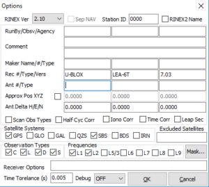
3. The auto detection of format normally works fine, but you can set it to ‘ublox‘ if you want to.
4. Under ‘Options’, you can fill in the receiver type under ‘Rec #’ as e.g. U-BLOX/LEA-6T/FW 7.03  and the Antenna type if it is a known one with a calibration (see the IGS14 ANTEX file; I don’t know of any single frequency L1 GPS antennas that have been calibrated) . This will allow correction for the antenna phase center but this is a <10cm effect. If your receiver can use GLONASS signals (the u-blox 6 can’t), you can tick that option. You can also put in an approximate position (in X, Y, Z format; use something like the NGS NCAT converter to convert). The CSRS-PPP can use this as a starting position to compare the solution to.
5. If you want trim off the start or the end of the data set (you can use the ‘Plot’ button to take a look), you can set these dates in the selectors at the top.

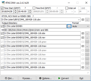
When you are done, you should have screen that look like the two above. Hit Convert to process the files and output the RINEX files. The main one we are interested in is the ‘OBS’ RINEX file. You can look at these in a text editor; they consist of a header and then a series of lines of data records. The data record starts with the time of observation and the specific satellites seen. This is then followed by the measurements (pseudorange, carrier phase, doppler shift and SNR); one line for each satellite.

Post processing for more precise GPS positions

To get more precise GPS positions than provided by the GPS itself, we need to do some post processing. The satellite orbits and clocks that are broadcast as part of the GPS signals are accurate to ~1 meter and ~5 ns respectively. Additionally, the estimates of the delay in path of the GPS signals caused by the ionosphere and the troposphere are not very accurate. The International GNSS Service receives and processes data from the GPS and GLONASS satellites at stations around the world. All of this data is then combined and used to make an increasingly accurate series of products. These products can be used to get more precise GPS positions from our data. CSRS-PPP is an online tool that can apply these products to our data to get a more accurate answer for the position. It’s also free to use.

Once you have registered on the website, you can log in and submit you data via the online form:

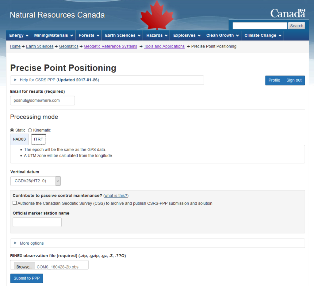
The RINEX OBS file can be uploaded as-is or compressed to produce a .zip or with gzip to reduce upload time. After a while (can be minutes to about an hour), you should get an email from the service with a zipfile of results. The PDF in the zipfile will give a nice summary of the dataset, showing the computed position and uncertainties, the difference to the estimated position  and a series of plots. The summary file will give more details about which satellite orbits & clocks and ionosphere and atmosphere models have been used. One thing to note: the results are only available on CSRS-PPP website for 48 hours. You should make sure to download the zipfile of results promptly.

The time from after the GPS data were taken until processing will determine what level of IGS products will be used:

IGS Data Products

Type		Accuracy	Delay	Updates
Broadcast	Orbits	~100 cm	real time	-
	Satellite clocks	~5 ns RMS
Ultra-Rapid (predicted part)	Orbits	~5 cm	real time	at 03, 09, 15, 21 UTC
	Satellite clocks	~3 ns RMS
Ultra-Rapid (observed part)	Orbits	~3 cm	After 3-9 hours	at 03, 09, 15, 21 UTC
	Satellite clocks	~0.15 ns RMS
Rapids	Orbits	~2.5 cm	After 17-41 hours	At 17 UTC each day
	Satellite clocks	~0.075 ns RMS
Finals	Orbits	~2.5 cm	After 12-18 days	Every Thursday
	Satellite clocks	~0.075 ns RMS

This shows that if you can wait about 12 hours for the Ultra-Rapids to become available, you can get a big improvement in the quality of the orbits and the clocks for the GPS satellites. Waiting approximately 2 days, allows you to get an another improvement with the use of the IGS Rapid products. While it seems that you have a long wait for the Finals with no improvement, this is not the whole story. The big advantage of the IGS Finals is that the satellite clocks are at 30 second (not 5 minute) intervals. This makes correcting the GPS receivers clock, which often drifts a lot, more accurate.

Results

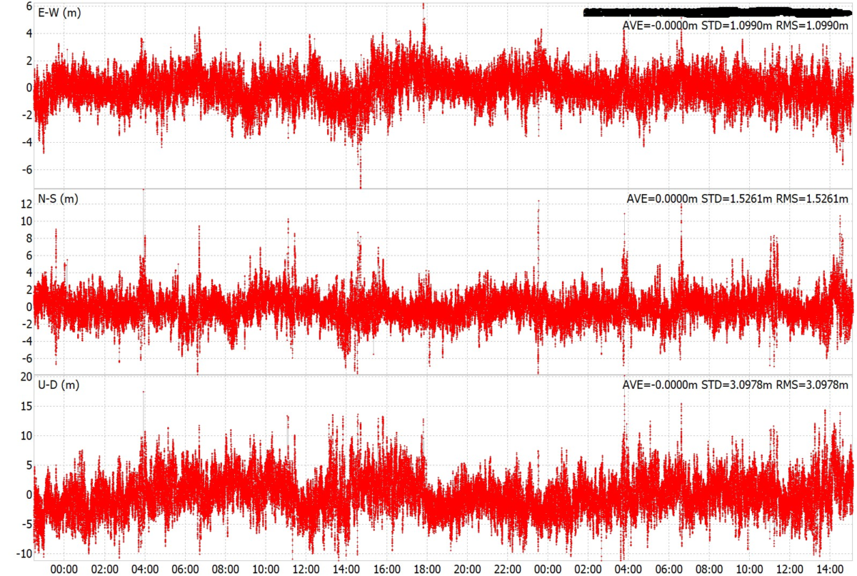
To give something of an example of what it possible, I will take a ~41 hour dataset that was recorded with a LEA-6T and the 53532A antenna in October 2017. Below is a plot of the solution post-processed with rtkpost using the broadcast ephemerides:

(The post processing was performed for this article as I foolishly didn’t save the original solution… The post processing was done using a combined file of the GPS satellite broadcast ephemerides from CDDIS for the recorded days. so should be very similar to what would have been seen in realtime)

The RMS values are approximately 1.1/1.5/3.1 meters in each of the East/North/Up directions. Combining them in quadrature produces an overall error of about 3.6m. The results after processing by CSRS-PPP with the IGS Finals are 0.089/0.105/0.217 meters in latitude, longitude and height respectively. This is reduction in the uncertainty by a factor of 12-14x which is pretty impressive.

1. Summary

   Hopefully this article has shown that with relatively modest equipment and use of clever software from clever people, it is possible to get very precise GPS positions. While they don’t match the results from survey equipment, which can normally achieve <2cm, we don’t do too badly with equipment that is a small fraction of the cost. In a later article, I will describe how you can setup a system to give you precise positions in real time.

In the meantime, if you have any questions or comments, please let me know by leaving a comment through the form at the bottom.

Acknowledgments

A lot of information on RTKLIB and how to use it came from https://rtklibexplorer.wordpress.com/ which is a great site with a lot of useful information. Definitely check it out if this stuff interests you.

Some of the information on the GPS signals and how receivers work, can from Jan Van Sickle’s online course on GPS and GNSS for Geospatial Professionals. In particular Lesson 1 on The GPS Signal has a lot of useful info on how GPS works.